Fe3+/Fe2+ model errors
This notebook shows the procedure we used to estimate errors on melt Fe3+/Fe2+ models. We use a validation dataset with measured melt Fe3+/Fe2+ ratios to estimate the accuracy and precision of the models included in MagmaPandas. The dataset can be downloaded here
import pandas as pd
import numpy as np
from scipy import optimize as opt
from scipy.interpolate import splrep, splev
from IPython.display import clear_output

import MagmaPandas as mp
import MagmaPandas.Fe_redox.Fe3Fe2_models as fe
from MagmaPandas.tools.model_errors import _error_func, _running_stddev

import matplotlib.pyplot as plt
Read the validation dataset and remove compositions not relevant for igneous petrology.
slags = ["KC1989", "K2000", "HI2007"]
hydrous = ["G2002", "G2003", "Bc2005"]
simplified_compositions = ["M2006"]#"BM2010"
inaccuracte_fO2 = ["SB2008"]

exclude = slags + simplified_compositions + inaccuracte_fO2

data = pd.read_csv("../../../src/MagmaPandas/model_calibrations/data/Fe3Fe2_calibration_data.csv")
data = data.replace([np.inf, -np.inf], np.nan)
data = data.query("ref not in @exclude")
Prepare data needed to run the models
models = mp.Fe3Fe2_models
results = {}

melts = mp.Melt(data, units="wt.%", datatype="oxide")
melts = melts[melts.elements]
melts.recalculate(inplace=True)

T_K = data["T_K"]
P_bar = data["P_bar"]
fO2 = data["fO2"]
These are all the models we are going to test, except for fixed.
print("\n".join(models))
armstrong2019
borisov2018
deng2020
fixed
hirschmann2022
jayasuriya2004
kress_carmichael1991
oneill2006
oneill2018
putirka2016_6b
putirka2016_6c
sun2024
zhang2017
Calculate Fe3Fe2 for the validation dataset with all models
for i, m in enumerate(models):

    if m == "fixed":
        continue
    model = getattr(fe, m)

    clear_output()
    print(f"model: {m}\n{i+1:03}/{len(models):03}")

    Fe3Fe2 = data[["ref", "run", "P_bar", "T_K", "fO2", "_Fe3Fe2",]].copy()
    Fe3Fe2["_Fe3Fe2_model"] = model.calculate_Fe3Fe2(melt_mol_fractions=melts.moles(), P_bar=P_bar, T_K=T_K, fO2=fO2)
    Fe3Fe2["delta"] = Fe3Fe2["_Fe3Fe2_model"] -Fe3Fe2["_Fe3Fe2"]
    Fe3Fe2 = Fe3Fe2.sort_values("_Fe3Fe2")

    results[m] = Fe3Fe2
model: zhang2017
013/013
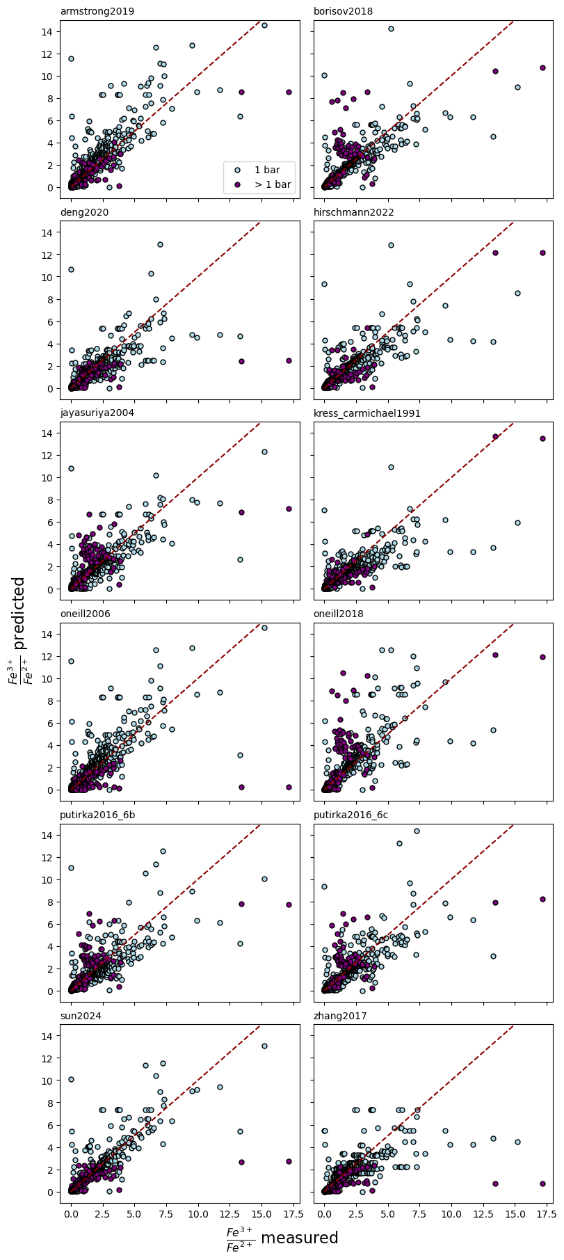
Plot showing model accuracies
qry = ""
pressure_cutoff = 1

fig, axs = plt.subplots(6, 2, figsize=(8,18), sharex=True, sharey=True, constrained_layout=True)

x_max = data["_Fe3Fe2"].max()

for i, (name, d) in enumerate(results.items()):

    d_lp = d.query("(P_bar <= @pressure_cutoff) & (_Fe3Fe2 < 20)")
    d_hp = d.query("(P_bar > @pressure_cutoff) & (_Fe3Fe2 < 20)")

    for df, c, l in zip((d_lp, d_hp), ("lightblue", "purple"), ("1 bar", "> 1 bar")):

        axs[i // 2, i % 2].plot(df["_Fe3Fe2"] , df["_Fe3Fe2_model"] , "o", mec="k", markersize=5, c=c, label=l)

    axs[i // 2, i % 2].plot([0, 15], [0, 15], "--", c="darkred", linewidth=1.5)
    axs[i // 2, i % 2].set_title(name, loc="left", size=10)


axs[0, 0].set_ylim(-1,15)
axs[0,0].legend()


fig.supxlabel("$\\frac{Fe^{3+}}{Fe^{2+}}$ measured", size=16)
fig.supylabel("$\\frac{Fe^{3+}}{Fe^{2+}}$ predicted", size=16)
plt.show()
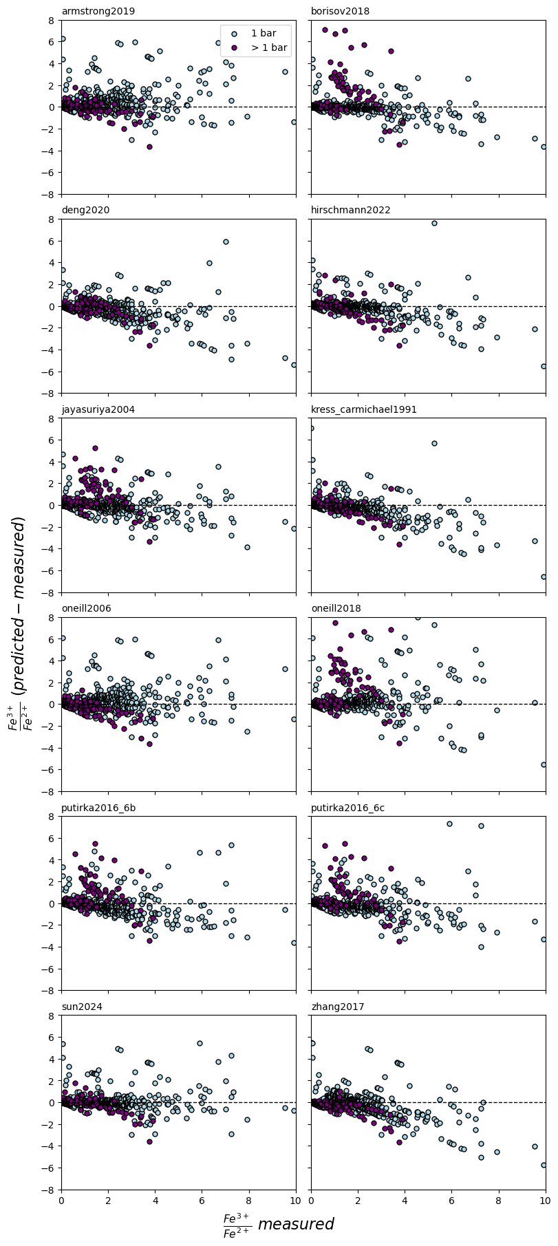
Alternative plot showing model accuracies
fig, axs = plt.subplots(6, 2, figsize=(8,18), sharey=True, sharex=True, constrained_layout=True)

for i, (name, d) in enumerate(results.items()):

    d_lp = d.query("P_bar <= @pressure_cutoff")
    d_hp = d.query("P_bar > @pressure_cutoff")


    for df, c, l in zip((d_lp, d_hp), ("lightblue", "purple"), ("1 bar", "> 1 bar")):

        axs[i // 2, i % 2].scatter(df["_Fe3Fe2"], df["delta"], marker="o", ec="k", c=c, s=5**2, label=l)

    axs[i // 2, i % 2].axhline(y=0, linestyle="--", linewidth=1., c="k")
    axs[i // 2, i % 2].set_title(name, loc="left", size=10)


axs[0,0].set_ylim(-8, 8)
axs[0,0].set_xlim(0, 10)
axs[0,0].legend()


fig.supylabel("$\\frac{Fe^{3+}}{Fe^{2+}}\ (predicted - measured)$", size=16)
fig.supxlabel("$\\frac{Fe^{3+}}{Fe^{2+}}\ measured$", size=16)

plt.show()
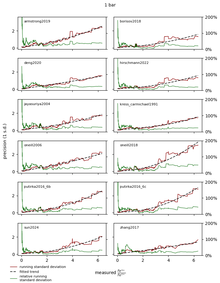
Plot showing model precision for experiments conducted at 1 bar. Precision is estimated from the standard deviation calculated in a moving window of 30 samples (i.e. the running standard deviation). Red lines show standard deviations in Fe3+/Fe2+ values (left y-axis) and green lines relative standard deviations are percentages (right y-axis). Both are plotted against the measured Fe3+/Fe2+ ratio on the x-axis. Both the absolute and relative standard deviations generally increase with measure Fe3+/Fe2+ ratios. We fitted mixed exponential + polynomial curves to the absolute standard deviations. The selected shapes for these curves are purely emperical. When MagmaPEC is run a 1 bar, it uses these curves to calculate errors during its error propagation model.
error_params = {}

mm = 1 / 25.4


from matplotlib.ticker import FuncFormatter

pressure_cutoff = 1

fig, axs = plt.subplots(6, 2, figsize=(185 * mm, 230 * mm), sharey=True, sharex=True, tight_layout=True)

sec_axs = np.empty(shape=axs.shape, dtype=axs.dtype)

for i, (name, d) in enumerate(results.items()):

    d_lp = d.query("P_bar <= @pressure_cutoff & (_Fe3Fe2 < 20)").sort_values("_Fe3Fe2")

    idx = d_lp["_Fe3Fe2_model"].dropna().index
    xvals, stddev = _running_stddev(d_lp.loc[idx, "_Fe3Fe2"], d_lp.loc[idx, "_Fe3Fe2_model"], boxsize=30)
    f_results = opt.curve_fit(f=_error_func, xdata=xvals, ydata=stddev, method="lm")
    error_params[name] = f_results[0]

    params = splrep(xvals, stddev, s=5)

    # axs[i // 2, i % 2].plot(d.query(qry)["_Fe3Fe2"] , d.query(qry)["_Fe3Fe2_model"] , "o", mec="k", markersize=3)
    axs[i // 2, i % 2].plot(xvals, stddev, "-", color="darkred", linewidth=1, label="running standard deviation")
    axs[i // 2, i % 2].plot(xvals, _error_func(xvals, *error_params[name]), "--", color="k", linewidth=1.5, alpha=0.8, label="fitted trend")

    # axs[i // 2, i % 2].plot(xvals, splev(xvals, params), "--", color="blue", linewidth=1.5, alpha=0.8)


    sec_axs[i // 2, i % 2] = axs[i // 2, i % 2].twinx()
    sec_axs[i // 2, i % 2].set_ylim(0,2)
    sec_axs[i // 2, i % 2].plot(xvals, stddev / xvals, "-", color="darkgreen", linewidth=1, alpha=0.8, label="relative running\nstandard deviation")


    axs[i // 2, i % 2].set_title(name, y=0.75, x=0.07, size=8, horizontalalignment="left")
    sec_axs[i // 2, i % 2].yaxis.set_major_formatter(FuncFormatter(lambda y, _: '{:.0%}'.format(y)))
    if (i % 2) == 0:
        sec_axs[i // 2, i % 2].set_yticklabels([])

h1, l1 = axs[0, 0].get_legend_handles_labels()
h2, l2 = sec_axs[0, 0].get_legend_handles_labels()
h = h1 + h2
l = l1 + l2
fig.legend(h, l, prop={"size": 8}, loc=(0.04, 0.0), frameon=False)

label_size = 10
fig.supxlabel("measured $\\frac{Fe^{3+}}{Fe^{2+}}$", size=label_size)
fig.supylabel("precision (1 s.d.)", size=label_size)
fig.suptitle("1 bar",va='bottom', size=label_size)

plt.show()
Store fitted mixed exponential + polynomial functions to the 1 bar running standard deviations. Coefficients are printed below
for i, (name, d) in enumerate(results.items()):

    d = d.query("P_bar <= 1 & (_Fe3Fe2 < 20)").sort_values("_Fe3Fe2")
    idx = d["_Fe3Fe2_model"].dropna().index

    xvals, stddev = _running_stddev(d.loc[idx, "_Fe3Fe2"], d.loc[idx, "_Fe3Fe2_model"], boxsize=30)
    f_results = opt.curve_fit(f=_error_func, xdata=xvals, ydata=stddev, method="lm")
    error_params[name] = f_results[0]

    print(f"\n{name}:\n{(np.array(f_results[0]),)}")
armstrong2019:
(array([1.82181137e-01, 3.23457995e-02, 9.74520443e-01, 1.02125866e+02]),)

borisov2018:
(array([0.07314587, 0.027771  , 0.4342864 , 3.39615194]),)

deng2020:
(array([2.02752244e-01, 5.39532829e-03, 9.86195285e-01, 2.56507793e+02]),)

hirschmann2022:
(array([0.06085686, 0.02986529, 0.55588899, 4.50065524]),)

jayasuriya2004:
(array([ 0.13422863,  0.00863356,  1.44302139, -7.44449788]),)

kress_carmichael1991:
(array([ 7.98973259e-02,  4.30191610e-03,  1.55259523e+00, -6.51661370e+00]),)

oneill2006:
(array([2.36503606e-01, 1.36742572e-02, 9.84395668e-01, 1.78234429e+02]),)

oneill2018:
(array([0.01227881, 0.08359905, 0.73796086, 8.78940681]),)

putirka2016_6b:
(array([5.60555414e-02, 5.28947436e-02, 9.83790217e-01, 1.59595205e+02]),)

putirka2016_6c:
(array([-3.88599903e-02,  7.76443966e-02,  9.81141740e-01,  1.22593221e+02]),)

sun2024:
(array([0.04935861, 0.0426917 , 0.53606871, 4.26521912]),)

zhang2017:
(array([1.66423440e-01, 7.69701987e-03, 9.85045614e-01, 2.31563095e+02]),)
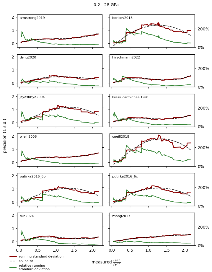
Plot showing model precision in experimentes conducted at pressures > 1 bar. The total pressure range of the included samples is 0.2 - 28 GPa Precision is estimated from the standard deviation calculated in a moving window of 30 samples (i.e. the running standard deviation). Red lines show standard deviations in Fe3+/Fe2+ values (left y-axis) and green lines relative standard deviations are percentages (right y-axis). Both are plotted against the measured Fe3+/Fe2+ ratio on the x-axis. For most models, standard deviations do not show systematic trends with measured Fe3+/Fe2+ ratios. Instead, standard deviations trends are often curved and decrease after an initial increase. This is especially apparant in the models that have been calibrated exclusively at 1 bar (Borisov et al. [2018], Jayasuriya et al. [2004], Putirka [2016] and O'Neill et al. [2018]), and shows that they do not capture Fe3+/Fe2+ variations with pressure.
We fitted splines to the absolute standard deviations. When MagmaPEC is run at pressures > 1 bar, it uses these fitted curves to calculate errors during its error propagation model.
error_params = {}


from matplotlib.ticker import FuncFormatter

pressure_cutoff = 1

fig, axs = plt.subplots(6, 2, figsize=(185 * mm, 230 * mm), sharey=True, sharex=True, tight_layout=True)

sec_axs = np.empty(shape=axs.shape, dtype=axs.dtype)

for i, (name, d) in enumerate(results.items()):

    d_hp = d.query("P_bar > @pressure_cutoff").sort_values("_Fe3Fe2")

    idx = d_hp["_Fe3Fe2_model"].dropna().index

    xvals, stddev = _running_stddev(d_hp.loc[idx, "_Fe3Fe2"], d_hp.loc[idx, "_Fe3Fe2_model"], boxsize=30)

    weights = np.ones(len(xvals))
    # weights[0]=10
    params = splrep(xvals.values, stddev, w=weights, s=3)
    # f_results = opt.curve_fit(f=_error_func, xdata=xvals, ydata=stddev, method="lm")
    # error_params[name] = f_results[0]


    # axs[i // 2, i % 2].plot(d.query(qry)["_Fe3Fe2"] , d.query(qry)["_Fe3Fe2_model"] , "o", mec="k", markersize=3)
    axs[i // 2, i % 2].plot(xvals.values, stddev, "-", color="darkred", linewidth=2, label="running standard deviation")
    axs[i // 2, i % 2].plot(xvals.values, splev(xvals, params), "--", color="k", linewidth=1.5, alpha=0.8, label="spline fit")

    sec_axs[i // 2, i % 2] = axs[i // 2, i % 2].twinx()
    sec_axs[i // 2, i % 2].set_ylim(0,3.5)
    sec_axs[i // 2, i % 2].plot(xvals, stddev / xvals, "-", color="darkgreen", linewidth=1.5, alpha=0.8, label="relative running\nstandard deviation")

    axs[i // 2, i % 2].set_title(name, y=0.8, x=0.03, size=8, horizontalalignment="left")
    sec_axs[i // 2, i % 2].yaxis.set_major_formatter(FuncFormatter(lambda y, _: '{:.0%}'.format(y)))
    if (i % 2) == 0:
        sec_axs[i // 2, i % 2].set_yticklabels([])


h1, l1 = axs[0, 0].get_legend_handles_labels()
h2, l2 = sec_axs[0, 0].get_legend_handles_labels()
h = h1 + h2
l = l1 + l2
fig.legend(h, l, prop={"size": 8}, loc=(0.04, 0.0), frameon=False)

label_size = 10
fig.supxlabel("measured $\\frac{Fe^{3+}}{Fe^{2+}}$", size=label_size)
fig.supylabel("precision (1 s.d.)", size=label_size)
fig.suptitle("0.2 - 28 GPa",va='bottom', size=label_size)

plt.show()
Store and print fited spline parameters
for i, (name, d) in enumerate(results.items()):

    d = d.query("P_bar > 1 & (_Fe3Fe2 < 20)").sort_values("_Fe3Fe2")
    idx = d["_Fe3Fe2_model"].dropna().index

    xvals, stddev = _running_stddev(d.loc[idx, "_Fe3Fe2"], d.loc[idx, "_Fe3Fe2_model"], boxsize=30)
    weights = np.ones(len(xvals))
    weights[0]=10

    print(f"\n{name}:\n{splrep(xvals, stddev, w=weights,s=3)}")
armstrong2019:
(array([0.05263158, 0.05263158, 0.05263158, 0.05263158, 2.16064117,
       2.16064117, 2.16064117, 2.16064117]), array([0.07460737, 0.63155495, 0.03894889, 0.77937143, 0.        ,
       0.        , 0.        , 0.        ]), 3)

borisov2018:
(array([0.05263158, 0.05263158, 0.05263158, 0.05263158, 0.59035243,
       2.16064117, 2.16064117, 2.16064117, 2.16064117]), array([0.00581678, 0.27693333, 1.48747235, 1.74215223, 0.50682697,
       0.        , 0.        , 0.        , 0.        ]), 3)

deng2020:
(array([0.05263158, 0.05263158, 0.05263158, 0.05263158, 2.16064117,
       2.16064117, 2.16064117, 2.16064117]), array([0.02618869, 0.59716833, 0.57214722, 0.25797173, 0.        ,
       0.        , 0.        , 0.        ]), 3)

hirschmann2022:
(array([0.05263158, 0.05263158, 0.05263158, 0.05263158, 2.16064117,
       2.16064117, 2.16064117, 2.16064117]), array([ 0.04061819,  0.87806539, -0.27681547,  0.57013273,  0.        ,
        0.        ,  0.        ,  0.        ]), 3)

jayasuriya2004:
(array([0.05263158, 0.05263158, 0.05263158, 0.05263158, 2.16064117,
       2.16064117, 2.16064117, 2.16064117]), array([0.06250386, 0.78697996, 1.9256632 , 0.49391875, 0.        ,
       0.        , 0.        , 0.        ]), 3)

kress_carmichael1991:
(array([0.05263158, 0.05263158, 0.05263158, 0.05263158, 2.16064117,
       2.16064117, 2.16064117, 2.16064117]), array([ 0.0676532 ,  0.72790213, -0.12375586,  0.58324872,  0.        ,
        0.        ,  0.        ,  0.        ]), 3)

oneill2006:
(array([0.05263158, 0.05263158, 0.05263158, 0.05263158, 2.16064117,
       2.16064117, 2.16064117, 2.16064117]), array([0.07265786, 0.69407306, 0.08782823, 0.73721276, 0.        ,
       0.        , 0.        , 0.        ]), 3)

oneill2018:
(array([0.05263158, 0.05263158, 0.05263158, 0.05263158, 0.59035243,
       2.16064117, 2.16064117, 2.16064117, 2.16064117]), array([0.01231242, 0.17101759, 1.97195171, 2.12089416, 0.89267432,
       0.        , 0.        , 0.        , 0.        ]), 3)

putirka2016_6b:
(array([0.05263158, 0.05263158, 0.05263158, 0.05263158, 2.16064117,
       2.16064117, 2.16064117, 2.16064117]), array([0.03474968, 0.73857782, 1.71983012, 0.40697316, 0.        ,
       0.        , 0.        , 0.        ]), 3)

putirka2016_6c:
(array([0.05263158, 0.05263158, 0.05263158, 0.05263158, 2.16064117,
       2.16064117, 2.16064117, 2.16064117]), array([0.02225772, 0.8568827 , 1.72229074, 0.36257493, 0.        ,
       0.        , 0.        , 0.        ]), 3)

sun2024:
(array([0.05263158, 0.05263158, 0.05263158, 0.05263158, 2.16064117,
       2.16064117, 2.16064117, 2.16064117]), array([ 0.06507369,  0.68064076, -0.00770687,  0.33039029,  0.        ,
        0.        ,  0.        ,  0.        ]), 3)

zhang2017:
(array([0.05263158, 0.05263158, 0.05263158, 0.05263158, 2.16064117,
       2.16064117, 2.16064117, 2.16064117]), array([0.02238626, 0.31307453, 0.44486454, 0.53007986, 0.        ,
       0.        , 0.        , 0.        ]), 3)