fO2

In this notebook we benchmark MagmaPandas fO2 codes by reproducing calculations and/or figures from literature. When possible, we compare MagmaPandas results to results from codes or data provided with the original publication of the model.

QFM

fO2 at QFM is calculated according to the method explained in van Gerve et al. (2004). This method is similar to the one implemented in the online fO2 app by Michael Anenburg. Here, the Anenburg implementation is compared to the one in MagmaPandas

from MagmaPandas.fO2 import QFM
from MagmaPandas.fO2 import IW
import pandas as pd
import numpy as np

import matplotlib.pyplot as plt
import geoplot as gp

mm = 1 / 25.4

We import data calculated with the Anenburg app at 1 bar and 10 kbar, over a 600 - 1800 K temperature range

fO2_anenburg_file = "./data/fO2/QFM_anenburg.csv"

fO2_QFM = pd.read_csv(fO2_anenburg_file)
T_K = fO2_QFM["T_K"]
P_bar = fO2_QFM["P_bar"]

fO2_QFM["fO2_magmapandas"] = QFM.calculate_fO2(T_K=T_K, P_bar=P_bar, logshift=0)

/Users/thomas/Dropbox/research/python/packages/MagmaPandas/src/MagmaPandas/EOSs/tools.py:55: RuntimeWarning: invalid value encountered in sqrt
  Q2 = np.where(t > tc, 0, np.sqrt((tc - t) / tc0))

gp.layout(colors=gp.colors.hollywood)

fig, axs = plt.subplots(1, 2, figsize=(180*mm, 85*mm), sharex=True, sharey=True)

for pressure, df in fO2_QFM.groupby("P_bar"):

    label = f"{pressure} bar" if pressure < 100 else f"{pressure / 1e4} GPa"

    axs[0].plot(df["T_K"], np.log10(df["fO2"]), "-", label=label)
    axs[1].plot(df["T_K"], np.log10(df["fO2_magmapandas"]), "-")

axs[0].legend(frameon=True, fancybox=False)
axs[0].set_title("Anenburg app")
axs[1].set_title("MagmaPandas")

fig.supxlabel("Temperature (K)")
fig.supylabel("log10 $f$O$_2$")
fig.suptitle("QFM")

plt.show()

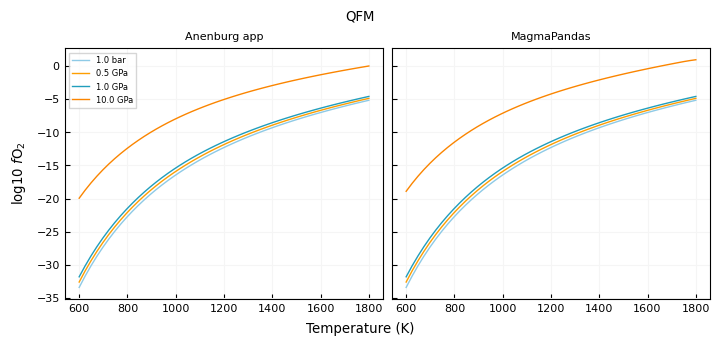
Note that there is a small difference in the pressure dependence visible at 10 GPa between the Anenburg app and MagmaPandas. This is most likely a result of the codes using different root-finding algorithms to solve the pressures of phase transitions. At the other calculated pressures, results are near identical.

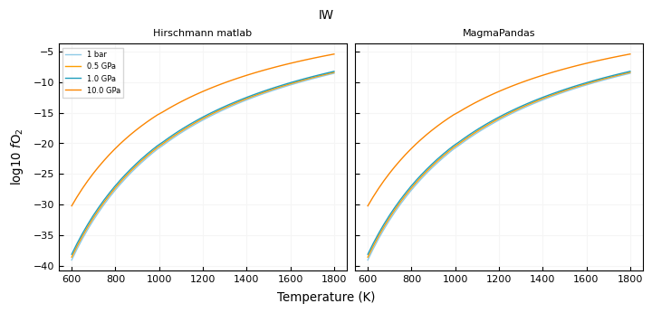
IW

fO2 at IW is calculated according to Hirschmann (2021). Here we compare Magmapandas results to those from the Matlabscript provided by the Hirschmann paper.

fO2_hirschmann_file = "./data/fO2/fO2_IW_hirschmann.csv"

fO2_IW = pd.read_csv(fO2_hirschmann_file)
T_K = fO2_IW["T_K"]
P_bar = fO2_IW["P_bar"]

fO2_IW["fO2_magmapandas"] = IW.calculate_fO2(T_K=T_K, P_bar=P_bar, logshift=0)

gp.layout(colors=gp.colors.hollywood)

fig, axs = plt.subplots(1, 2, figsize=(180*mm, 85*mm), sharex=True, sharey=True)

for pressure, df in fO2_IW.groupby("P_bar"):

    label = f"{pressure} bar" if pressure < 100 else f"{pressure / 1e4} GPa"

    axs[0].plot(df["T_K"], np.log10(df["fO2"]), "-", label=label)
    axs[1].plot(df["T_K"], np.log10(df["fO2_magmapandas"]), "-", label=label)


axs[0].legend(frameon=True, fancybox=False)
axs[0].set_title("Hirschmann matlab")
axs[1].set_title("MagmaPandas")

# axs[1].set_ylim(-0.1, 0.1)

fig.supxlabel("Temperature (K)")
fig.supylabel("log10 $f$O$_2$")
fig.suptitle("IW")

plt.show()