Model selection and calibration datasets

To calculate realistic melt Fe3Fe2 ratios and Kd, it is important to select a model that has been calibrated with melt compositions and PT conditions similar to those of your own melts. This example shows how to plot and compare melt compositions of experiments included in datasets used to calibrate the models included in MagmaPandas.

MagmaPandas includes the calibration datasets for all Fe3/Fe2 models. Unfortunately, for many ol-melt Fe-Mg Kd models it is either not clearly explained which data were included in their calibration, or the data are not accessible. Because of this, MagmaPandas only includes calibration datasets for the Blundy et al. [2020] and Sun and Dasgupta [2020] Kd models.

from MagmaPandas.model_calibrations import plot_calibration, plot_calibration_PT, get_calibration_data
import matplotlib.pyplot as plt
import geoplot as gp
import MagmaPandas as mp

With the function get_calibration_data from the model_calibration module in Magmapandas you can retrieve model calibration datasets. Currently, this is only implemented for melt Fe3Fe2, which you need to pass to the parameter argument. Without supplying any other argument, the function return the calibration dataset for the model currently selected in the configuration. In this case, that is the sun2024 model.

print(mp.configuration)
calibration_data_Fe3Fe2 = get_calibration_data(parameter="Fe3Fe2")
calibration_data_Fe3Fe2

################## MagmaPandas ###################
##################################################
General settings__________________________________
fO2 buffer.....................................QFM
ΔfO2.............................................1
Melt Fe3+/Fe2+.............................sun2024
Kd Fe-Mg ol-melt........................toplis2005
Melt thermometer....................putirka2008_15
Volatile solubility model.......iaconomarziano2012
Volatile species.............................mixed
##################################################

	ref	run	SiO2	TiO2	Al2O3	MgO	CaO	Na2O	K2O	P2O5	MnO	CoO	NiO	Pb	FeO	T_K	fO2	_Fe3Fe2	P_bar
0	A2019	S6776	56.40	3.53	13.30	2.77	7.49	4.40	0.63	0.0	NaN	NaN	NaN	NaN	8.647177	2573.15	1.181990e+07	17.138110	230000.0
1	A2019	S6606	57.76	2.47	15.30	1.77	6.39	4.80	1.03	0.0	NaN	NaN	NaN	NaN	6.523624	2573.15	1.181990e+07	13.425202	230000.0
2	A2019	Z1850	45.06	0.75	18.33	10.20	12.87	2.23	0.00	0.0	NaN	NaN	NaN	NaN	8.098292	2473.15	1.121269e+06	1.024902	180000.0
3	A2019	Z1791	50.22	2.37	15.70	8.57	12.34	3.30	0.00	0.0	NaN	NaN	NaN	NaN	7.243473	2473.15	1.121269e+06	0.590352	180000.0
4	A2019	Z1626	52.45	2.40	14.47	2.22	6.53	5.17	0.58	0.0	NaN	NaN	NaN	NaN	13.785093	2473.15	9.320000e-04	0.052632	150000.0
...	...	...	...	...	...	...	...	...	...	...	...	...	...	...	...	...	...	...	...
1215	Z2016	VF59	59.66	2.76	14.43	2.05	7.18	4.16	1.10	0.0	NaN	NaN	NaN	NaN	9.349029	1623.15	6.606930e-04	0.772735	1.0
1216	Z2016	VF81	59.81	3.00	14.46	2.15	7.72	3.37	1.02	0.0	NaN	NaN	NaN	NaN	8.548197	1623.15	1.050000e-07	0.118944	1.0
1217	Z2016	VF88	60.18	2.81	14.45	2.04	7.25	3.55	0.90	0.0	NaN	NaN	NaN	NaN	9.555985	1623.15	5.500000e-07	0.191611	1.0
1218	Z2016	VF49	60.25	2.95	14.62	2.17	7.70	3.07	1.00	0.0	NaN	NaN	NaN	NaN	8.179275	1623.15	2.340000e-09	0.118318	1.0
1219	Z2016	VF35	60.30	2.91	14.66	2.06	7.38	3.38	1.10	0.0	NaN	NaN	NaN	NaN	9.106080	1623.15	8.510000e-09	0.069633	1.0

1080 rows × 19 columns

For the default Kd model (toplis2005) the calibration dataset is not available and the get_calibration_data function raises an error.

get_calibration_data(parameter="Kd")

---------------------------------------------------------------------------
RuntimeError                              Traceback (most recent call last)
Cell In[3], line 1
----> 1 get_calibration_data(parameter="Kd")

File ~/Dropbox/research/python/packages/MagmaPandas/src/MagmaPandas/model_calibrations/plot_calibration.py:66, in get_calibration_data(parameter, model)
     63 datasets = calibration_datasets[model]
     65 if datasets is None:
---> 66     raise RuntimeError(
     67         f"The calibration dataset is not available for {model}. Please refer to the original publication."
     68     )
     70 data = calibration_data.query("ref in @datasets")
     72 return data

RuntimeError: The calibration dataset is not available for toplis2005. Please refer to the original publication.

By supplying a name to the model argument you can get calibration dataset for other models. The Fe3Fe2 and Kd models you can choose from are listed in the mp.Fe3Fe2_models and mp.Kd_ol_FeMg_models variables respectively.

print("Fe3Fe2 models: ", mp.Fe3Fe2_models, "\nKd models: ", mp.Kd_ol_FeMg_models)

calibration_data_Kd = get_calibration_data(parameter="Kd", model="blundy2020")
calibration_data_Kd

Fe3Fe2 models:  ['armstrong2019', 'borisov2018', 'deng2020', 'fixed', 'hirschmann2022', 'jayasuriya2004', 'kress_carmichael1991', 'oneill2006', 'oneill2018', 'putirka2016_6b', 'putirka2016_6c', 'sun2024', 'zhang2017'] 
Kd models:  ['blundy2020', 'fixed', 'putirka2016_8a', 'putirka2016_8b', 'putirka2016_8c', 'putirka2016_8d', 'saper2022', 'sun2020', 'toplis2005']

	ref	run	SiO2	TiO2	Al2O3	FeO	MnO	MgO	CaO	Na2O	...	CO2	total	_Fe3Fetotal	T_K	P_bar	_Fe3Fe2	olivine_forsterite	fO2	kd_FeTMg	kd_Fe2Mg
0	Bl2020	10	43.30	1.02	14.00	8.71	0.18	10.53	11.99	2.050	...	NaN	97.28	NaN	1523.15	13000	NaN	0.905000	NaN	0.222	NaN
1	Bl2020	12	44.01	1.15	15.19	8.85	0.20	9.60	10.53	2.710	...	NaN	97.60	NaN	1473.15	13000	NaN	0.918000	NaN	0.167	NaN
2	Bl2020	15	43.61	0.97	13.61	9.14	0.19	10.90	12.36	2.180	...	NaN	97.71	NaN	11538.15	13000	NaN	0.914000	NaN	0.195	NaN
3	Bl2020	22	44.05	1.00	13.78	9.02	0.21	10.39	12.07	2.250	...	NaN	96.69	NaN	1538.15	10000	NaN	0.949000	NaN	0.107	NaN
4	Bl2020	23	43.78	0.91	12.62	8.86	0.17	12.32	12.30	1.870	...	NaN	97.12	NaN	1548.15	7000	NaN	0.943000	NaN	0.144	NaN
...	...	...	...	...	...	...	...	...	...	...	...	...	...	...	...	...	...	...	...	...	...
89	M2006	FDA3-1.5-00	46.51	NaN	11.69	12.06	1.45	14.00	11.48	NaN	...	NaN	NaN	NaN	1573.15	1	0.800000	0.957000	2.090000e-01	NaN	0.463930
90	M2006	FDA3-10	42.52	NaN	14.05	16.98	1.03	12.25	12.17	NaN	...	NaN	NaN	NaN	1573.15	1	0.118000	0.817900	1.000000e-08	NaN	0.324638
91	M2006	FDA3-2-00	45.07	NaN	11.52	12.13	2.04	14.26	11.39	NaN	...	NaN	NaN	NaN	1573.15	1	0.800000	0.965400	2.090000e-01	NaN	0.375529
92	Ma2011	26	46.33	1.49	8.80	12.31	0.17	23.90	7.36	0.094	...	NaN	NaN	NaN	1773.15	1	0.171265	0.922940	3.090000e-06	NaN	0.338426
93	Ma2011	39	46.71	1.67	9.86	13.80	0.17	19.51	9.15	0.400	...	NaN	NaN	NaN	1669.15	1	0.584416	0.969658	2.089296e-01	NaN	0.124945

94 rows × 26 columns

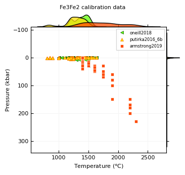
The function plot_calibration_PT plots pressures as a function of temperature for experiments from the calibration datasets. The parameter you want to show needs to be passed as an argument, so here we use Fe3Fe2. Without any other arguments, the plot will include all available models.

plot_calibration_PT(parameter="Fe3Fe2")

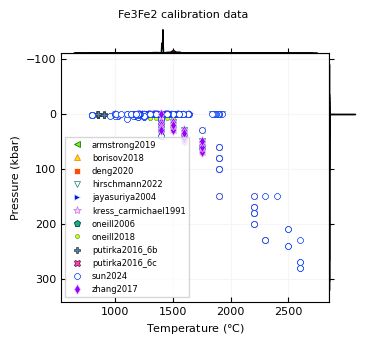
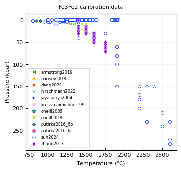
The plot includes kernel density estimates (kde) on the x- and y-axis. For models calibrated in a narrow pressure or temperature range, these kde’s are very narrow and do not provide much information. The kde’s can be removed by passing False to the sidekde argument. Note that many models use some of the same experiments in their calibrations, so many symbols overlap.

ax = plot_calibration_PT(parameter="Fe3Fe2", sidekde=False)

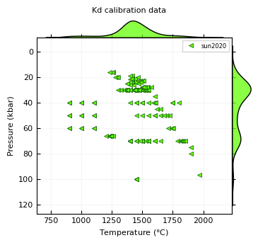
By passing a model name, or a list of model names to the models argument, one or more models can be plotted. Available models are listed in the mp.Fe3Fe2_models variable.

print(mp.Fe3Fe2_models)
plot_calibration_PT(parameter="Kd", models="sun2020")

['armstrong2019', 'borisov2018', 'deng2020', 'fixed', 'hirschmann2022', 'jayasuriya2004', 'kress_carmichael1991', 'oneill2006', 'oneill2018', 'putirka2016_6b', 'putirka2016_6c', 'sun2024', 'zhang2017']

plot_calibration_PT(parameter="Fe3Fe2", models=["oneill2018", "putirka2016_6b", "armstrong2019"])

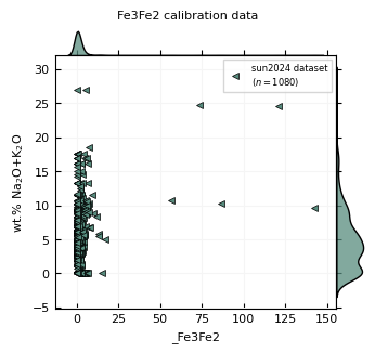
The function plot_calibration plots melt compositions of experiments included in calibration datasets. Again, the name of the parameter needs to be passed to the parameter argument. Without supplying any other argument, the function will show the calibration dataset for the model currently selected in the configuration. In this case, that is the sun2024 Fe3Fe2 model (see above).

x- and y-axis elements or other variables (e.g. fO2, Kd, Fe3Fe2 etc.) need to be passed as strings to the x_elements and y_elements parameters. If you provide a list of elements, they will be summed in the plot. In the example below, Na2O and K2O are plotted as a sum on the y-axis. Names have to be the same as the columns in calibration_data - the options for Fe3Fe2 and Kd datasets are listed below.

print("Fe3Fe2 options: ", list(calibration_data_Fe3Fe2.columns), "\nKd options: ", list(calibration_data_Kd.columns))

Fe3Fe2 options:  ['ref', 'run', 'SiO2', 'TiO2', 'Al2O3', 'MgO', 'CaO', 'Na2O', 'K2O', 'P2O5', 'MnO', 'CoO', 'NiO', 'Pb', 'FeO', 'T_K', 'fO2', '_Fe3Fe2', 'P_bar'] 
Kd options:  ['ref', 'run', 'SiO2', 'TiO2', 'Al2O3', 'FeO', 'MnO', 'MgO', 'CaO', 'Na2O', 'K2O', 'P2O5', 'Cr2O3', 'CoO', 'NiO', 'H2O', 'CO2', 'total', '_Fe3Fetotal', 'T_K', 'P_bar', '_Fe3Fe2', 'olivine_forsterite', 'fO2', 'kd_FeTMg', 'kd_Fe2Mg']

melt_file = "./data/melts.csv"

melt = mp.read_melt(melt_file, index_col=["name"])

x = "_Fe3Fe2"
y = ["Na2O", "K2O"]

plot_calibration(
    parameter="Fe3Fe2",
    x_elements=x,
    y_elements=y,
    sidekde=True
)

plt.show()

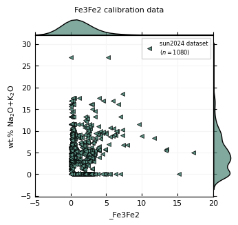
plot_calibration returns the pyplot figure and axis. If you assign them to variables, you can edit the figure or axes. Below we change the limits of the x-axis.

melt_file = "./data/melts.csv"

melt = mp.read_melt(melt_file, index_col=["name"])

x = "_Fe3Fe2"
y = ["Na2O", "K2O"]

fig, ax = plot_calibration(
    parameter="Fe3Fe2",
    x_elements=x,
    y_elements=y,
    sidekde=True
)
ax.set_xlim(-5,20)

plt.show()

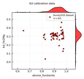
To change the symbols of the plotted points, pass a dictionary to the calibration_props argument. This dictionary gets passed to the plot method of pyplot as keyword arguments. Here we plot olivine forsterite content against measured Kd Fe2-Mg values.

x = "olivine_forsterite"
y = "kd_Fe2Mg"

plot_calibration(
    parameter="Kd",
    models="blundy2020",
    x_elements=x,
    y_elements=y,
    sidekde=True,
    calibration_props={"color": "red", "markersize":5}
)

plt.show()

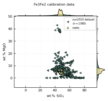
You can plot your own melt compositions together with the calibration data by passing them as a pandas dataframe to the melts argument. Column names for oxides also have to be the same as in calibration_data. Here the y-axis is changed to show MgO contents.

melt_file = "./data/melts.csv"

melt = mp.read_melt(melt_file, index_col=["name"])

x = "SiO2"
y = "MgO"

plot_calibration(
    parameter="Fe3Fe2",
    x_elements=x,
    y_elements=y,
    melts=melt,
    sidekde=True
)

plt.show()

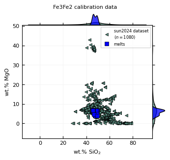
To change the symbols of the plotted melt points, pass a dictionary to the melt_props argument. This dictionary gets passed to the plot method of pyplot as keyword arguments.

x = "SiO2"
y = "MgO"

plot_calibration(
    parameter="Fe3Fe2",
    x_elements=x,
    y_elements=y,
    melts=melt,
    sidekde=True,
    melt_props={"color": "blue", "markersize":6, "marker":"s"}
)

plt.show()

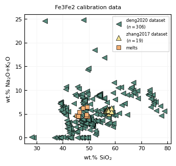
Here is a similar plot, with multiple models and without kde’s.

x = "SiO2"
y = ["Na2O", "K2O"]

plot_calibration(
    parameter="Fe3Fe2",
    models=["deng2020", "zhang2017"],
    melts=melt,
    x_elements=x,
    y_elements=y,
    sidekde=False,
    melt_props={"markersize": 6},    
    calibration_props={"markersize":7}
)

plt.show()

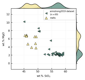
If you want to have more control over the plot, you can also create your own figure with matplotlib and pass the axis to the ax argument of plot_calibration.

mm = 1 / 25.4
gp.layout(colors=gp.colors.campfire)

x = "SiO2"
y = "MgO"

fig, ax = plt.subplots(figsize=(85 * mm, 80 * mm))

calibration, *_ = plot_calibration(
    parameter="Fe3Fe2",
    models="armstrong2019",
    ax=ax,
    x_elements=x,
    y_elements=y,
    melts=melt,    
    calibration_props={"mec": "k", "ms": 6},
    melt_props={"mec": "k", "ms": 7},
)

ax.set_xlabel(f"wt.% {gp.subscript_numbers(x)}")
ax.set_ylabel(f"wt.% MgO")

ax.legend(frameon=True)

plt.show()